Using NLTK to Recommend Books

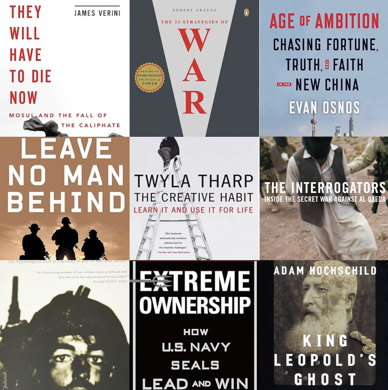
I read 12 books in 2023 which I made into a CSV file, including columns such as the title, author(s), genre, and the blurb. This process of collecting the data myself reminded me of the difficulties involved in data sourcing during my time at the U.S. Census Bureau.

I first analyzed the trends in my 2023 reading list by calculating the readability score of each book. Then I used the dataset of my 2023 reading list as a training set to recommend books most similar in a test dataset based on the blurbs.

1. Based on the blurb (description) what is the median readability score by genre?

I preprocessed the dataframe to explode the genre column into individual rows. I then applied the flesh_reading_ease library to the each blurb. The tool determines a score by taking into account the total words per sentence and total syllables per word. I decided to use the median of the readability scores instead of the average for each genre due to the nature of the small dataset which could be easily skewed by an outlier.

Key Observations:
• The genres that were scored as less difficult to read are in line with books targeted towards a wider audience such as self-help and creative
• The one genre that was common across all 12 books I read was nonfiction therefore it is the score that demonstrates the median overall readability score

Hover over the sunchart to explore the scores

Calculating the readability by genre

# (1) Extracting the genres from the "genre" column with .explode()
# This will cause a repeat of Books in order to analyze by genre, each genre will have its own row per book
books23_expanded = books23.assign(Genre=books23['Genre'].str.split(',')).explode('Genre') # use commas as split point
books23_expanded['Genre'] = books23_expanded['Genre'].str.lower()

# (2) Strip extra spaces from the genres
books23_expanded['Genre'] = books23_expanded['Genre'].str.strip()

# (3) Define a function to use on the "blurb" column
def calc_readability(text):
    return textstat.flesch_reading_ease(text)
# Note the flesch reading score is formatted as follows: 
# 90 - 100         5th grade         very easy 
# 80 - 90          6th grade         easy 
# 70 - 80          7th grade         fairly easy 
# 60 - 70          8-9 grades        standard 
# 50 - 60         10 - 12th grades   fairly difficult 
# 30 - 50          college           difficult
# 0 - 30           college grade     very difficult 
# the calculation considers factors such as total words/total sentences + total syllables/total words

# (4) Apply to the "blurb" column of df
# Assign results to new df column "Readability_Score"
books23_expanded['Readability_Score'] = books23['Blurb'].apply(calc_readability) # each book duplicate will repeat the overall score 

# (5a) Analyze the results 
# (5b) Calculate the average readability score by genre
average_scores_by_genre = books23_expanded.groupby('Genre')['Readability_Score'].mean()

# Verify results: 
# books23_expanded
average_scores_by_genre
# books23

# (5c) What is the median reading score by genre? 
med_genre_scores =books23_expanded.groupby('Genre')['Readability_Score'].median().sort_values()

# (6) Convert back to a dataframe by putting an index back 
med_genre_scores = med_genre_scores.reset_index() # only run once

Visualizing the results with a sunchart

# (1) Visualizing the median readability score by genre: 
med_genre_scores

# (2) print(med_genre_scores['Readability_Score'])

# (3a) Use the plotly express px sunbursts plot type 
sun_chart = px.sunburst(med_genre_scores, path = ['Genre'], # the titles of each piece 
                        values = 'Readability_Score', # set values to the readability score
                        title = 'Evaluating My 2023 Reading list:<br><sub> Median Readability Score by Genre</sub>',
                        color='Readability_Score', # color by score
                        color_continuous_scale = 'Blackbody') # use built-in gradient where red is on the more difficult side 
# (3b) Increase the size of the chart
sun_chart.update_layout(
    title={
        'x': 0.5,  # center the title horizontally
        'xanchor': 'center',
        'yanchor': 'top',
        'font': {
            'size': 24,
            'color': 'black',
            'family': 'Arial' # set font family
        }
    },
    coloraxis_colorbar_title_text='Flesch Readability Score',
    width=800,  # Set the width of the figure
    height=600)

# (3c) Change the hover results 
sun_chart.update_traces(
    hovertemplate='Genre:%{label}<br>Median Readbility Score: %{value}') # simplify the hover to just Genre and Score
sun_chart.show()

# (4) Export the visual to be an HTML for my website
div = pyo.plot(sun_chart, include_plotlyjs=False, output_type='div')
with open("MedianReadability_byGenre.html", "w") as file:
    file.write(div)

Preprocessing the text from the blurbs involved converting all characters to lowercase, removing puncutation, assigning stop words, tokenizing the text to individual words, removing stop words, and applying the lemmatize library to find the stem of words. I made this preprocessing step into a function in order to call it for each dataset.

After preprocessing the blurbs, I utilized the TfidfVectorizer from sklearn in order to convert the text into numerical values in a vector space model. The Term Frequency-Inverse Document Frequency (TF-IDF) has two parts the former measures the frequency of each term then the later applies a weight or importance to each term-the logarithm of the total number of documents in the corpus divided by the number of documents containing the term. The logarithm is taken of the ratio in order to minimize the terms that occur too frequently. This means that a higher IDF score represents a term that occurs less frequently across documents.

The matrices were then used to determine the cosine similarity first between the training set to the training set in order to verify the program was operating accurately then between the training set and the test set to recommend books. The cosine_similarity function employs the dot product of the two matrices divided by the product of the magnitudes. It is key to only apply the fit_transform() to the training set and then the transform() to the testing set in order to produce matrices that are compatible mxn to apply a cosine_similarity(). Initially, I mistakenly applied fit_transform() to both the training and testing set which resulted in an error “Incompatible dimension for X and Y matrices.”

Another key modification I applied was changing the parameters of the cosine_similarity() function to find the most similar books based on all the books as an aggregate via mean score method as opposed to one book from my reading list at a time. This step was important because applying the cosine similarity based on one book provided less accurate recommendations and the results from each input book were vastly different. For example, one attempt with only a single book which mentioned courage in the blurb resulted in a children’s book on courage making the recommended list of similar books.

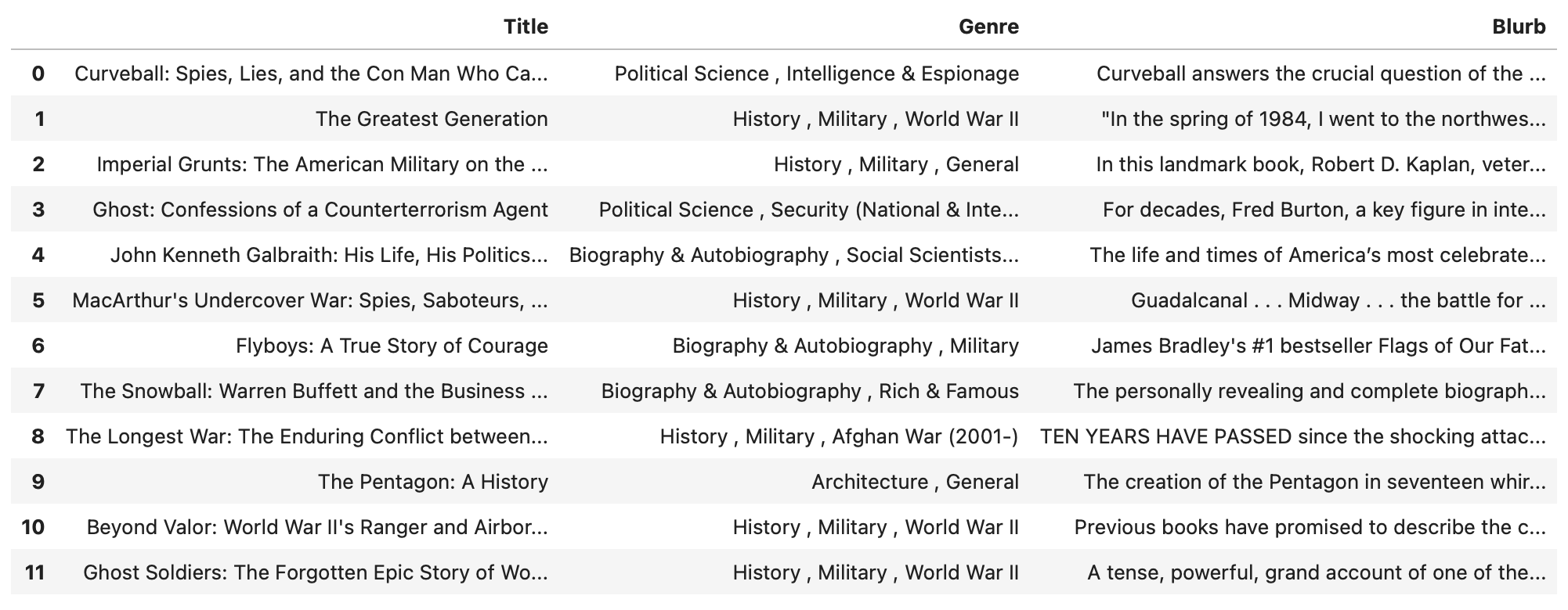
The final judgement, determining if I would read the books recommended. Once a comprehensive dataframe of recommended books was produced-sorted in descending order by scores-I filtered out all fiction genre titles and duplicates to best suit my personal reading preferences. Then I reviewed the top 12 books by title and description. I can confirm that I would indeed read the 12 books produced by my NLTK program.

Key Observations:
• Applying the right transformation to produce matrices is key to then utilizing the cosine similarity, which must be of the same mxn because the function utilizes the dot product
• Even though I only trained the model based on the blurbs from my reading dataset, the genres between the two dataframes demonstrate a lot of similarities such as History, Military, and War
• The titles and descriptions of the top 12 books recommended encapsulate similarities not just in stand alone words, but also elicit phrases, themes, and time periods similar to the books I read

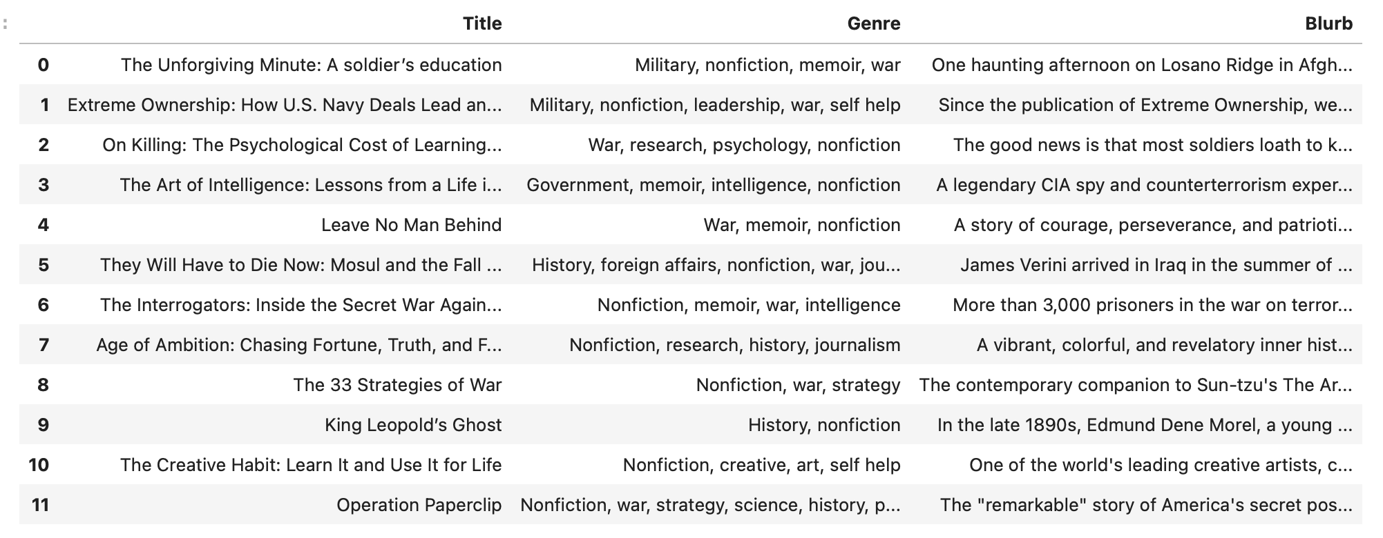
The 2 dataframes

The 12 books I read in 2023:

The top 12 books recommened for me:

Preprocessing the text

# (1a) Preprocessing the text from the blurbs
# (1b) Convert all letters to lowercase and assign to new series
books_23_lc = books23['Blurb'].str.lower() # must use str to apply method to series

# (1c) Function that removes punctuation, stopwords, and applies 'stemming'
# to find the root word and meaning
# Define the txt preprocessing function
def preprocess_txt(txt):
    
    # (1.1) Remove punctuation using 'string' module
    txt = txt.translate(str.maketrans('', '', string.punctuation)) # remove periods, commas, etc. 
    
    # (1.2) Remove stopwords, use NLTK library and assign to stop_words as a set
    stop_words = set(stopwords.words('english')) 
    indv_words = word_tokenize(txt) # divide into individual words, assaign as indv_words
    txt = ' '.join([word for word in indv_words if word not in stop_words]) # iterate through each word checking id it is in stop_words
                                                                       # Rejoin the text if the words from indv_words are not stop_words

    # (1.3) Apply Stemming to find the base of words
    stemm = WordNetLemmatizer() # use NLTK library to find stems of words 
    indv_words = word_tokenize(txt) # tokenize as indv words again
    txt = ' '.join([stemm.lemmatize(word) for word in indv_words]) # iterate through each word and apply 
    
    return txt

# (1d) Apply the preprocessing function to the series
books_23_lc = books23['Blurb'].apply(preprocess_txt)

# books_23_lc # Verify work

# (2a) Convert blurbs to numerical data via TF-IDF Vectorizer from sklearn

# (2b) Initialize TFIDF to determine word frequency and weight
vectorizer = TfidfVectorizer()

# (2c) Transform the preprocessed series to TFIDF matrix
matrix = vectorizer.fit_transform(books_23_lc) # learn vocabulary and idf

# matrix # verify work

# (3a) Calculate cosine simularity (from -1 to 1) 
# Apply previous matrix to itself, this will only determine which books are most similar within the set itself  
cosine_matrix = cosine_similarity(matrix, matrix)

# (3b) Function to pair similarity scores
def find_most_similar_books(books, cosine_matrix, top_n=5):
    # Get the pairwise similarity scores of all books with the given book
    sim_scores = list(enumerate(cosine_matrix[books]))
    
    # Sort the books based on the similarity scores
    sim_scores = sorted(sim_scores, key=lambda x: x[1], reverse=True)
    
    # Get the scores of the most similar books (excluding the book itself)
    sim_scores = sim_scores[1:top_n + 1]
    
    # Get the book indices for sim_scores
    books = [i[0] for i in sim_scores]
    
    return books

# Apply function: determine the 2 most similar books to the nth book in my dataset
most_similar_books = find_most_similar_books(2, cosine_matrix, top_n=2)
# most_similar_books # Verify work

Preparing the test dataset

# Set up Test Books Dataframe
# (1) Read in the dataset
books_testset = pd.read_csv("BooksDataset.csv")

# (2) Filter for books that have a dataset using a mask
testset_mask = books_testset['Description'].notna() # remove NaN Description observations

# (3) Only use the books that have a description 
books_wdescription = books_testset[testset_mask].copy()

# (4) Preprocess the dataframe using the same function as before 'preprocess_txt' 
books_wdescription['Processed_Des']  = books_wdescription['Description'].apply(preprocess_txt)

# (5) Convert blurbs to numerical data via TF-IDF Vectorizer from sklearn
# because this is not our training set but rather a test set, only use transform 
testset_matrix = vectorizer.transform(books_wdescription['Processed_Des'])

Verifying that the two matrices are compatible mxn for dot product

# Before calculating the cosine coefficient for the two matrices, ensure that the columns are the same value 
# use .shape()
# print(matrix.shape) # 11x930
# print(testset_matrix.shape) # 70213x930

# (6) Use cosine coefficient to calculate similarity between the TFIDF vectors from the testset_matric
# compared to my own reading dataframe matrix
cosine_2sets = cosine_similarity(testset_matrix, matrix)

# (1a) Attempt #1, find the top 10 books in the random dataset most similar to one of my personal books
top_similar = cosine_2sets[:, 3].argsort()[-10:][::-1]  # Assuming you're interested in the first book

# (1b) Locate the books via index using .iloc[]
recommended_books = books_wdescription.iloc[top_similar]

# (1c) Print the results and inspect the accuracy by reading the titles and descriptions
print(recommended_books[['Title', 'Description']])

# Observations: 
# As I change the book that the the model is using to recommend the most similar books, the results vary greatly
# I will instead try an aggregate method to find books that match a subset or the whole set of books from my reading list

# (2a) Attempt #2, recalculate the cosine similarity, but this time set a subset from the personal books matrix
similarity_set = cosine_similarity(testset_matrix, matrix[:11])

# (2b) Use the average similarity of each book from the test set to my personal set
avg_similarity_set = similarity_set.mean(axis=1)

# (3a) Extract the top 5 via index and assign to new dataframe
# Use 1000 because we will then filter and modify the results to best recommend books
avg_top = avg_similarity_set.argsort()[-1000:][::-1] # argsort to sort the indices, -1000 slices the last 1000 books, -1 to reverse the array
books_recommended_byset = books_wdescription.iloc[avg_top].copy() # assign to new df based on top 5 similarity scores sliced

# (3b) Print the Title and Description columns of the resulting dataframe and inspect results
# print(books_recommended_byset[['Title', 'Description']])

# Observations: 
# Based on the titles and descriptions, I can confirm that I would read the top 5-10 books, BUT
# there are too many fiction books and I have a strong preference for nonfiction

# (4) Save the similarity scores as new column 
books_recommended_byset['Similarity_Score'] = avg_similarity_set[avg_top]
# (4b) Sort the dataframe based on the new column in descending order
books_recommended_byset = books_recommended_byset.sort_values(by='Similarity_Score', ascending=False)

# Filter out the fiction genre

# Rename the columns from Category to Genre
books_recommended_clean = books_recommended_byset.rename(columns={'Category':'Genre'})

# Extract the genres from the 'Genre' column with .explode()
recommended_nonfiction = books_recommended_clean[~books_recommended_clean['Genre'].str.contains('Fiction', case=False, na=False)]

# Filter for unique titles, extract top 12
recommended_nonfiction_unique = recommended_nonfiction.drop_duplicates(subset=['Title'], keep='first')
recommended_nonfiction_unique = recommended_nonfiction_unique.head(12)

Dataset source:
https://www.kaggle.com/datasets/elvinrustam/books-dataset

Using NLTK to Recommend Books

Analyzing the books I read in 2023 to recommend new books: